The Phenotype Genotype Reference Map (PGRM) is a set of associations from the (NHGRI-EBI GWAS catalog. The pgrm package enables users to calculate replication related measures on test cohorts.
This vignette shows how replication measures can be calculated based on summary statistics from a test cohort. (To generate summary statistics from raw data, see the run_PGRM_assoc() function.)
Load GWAS summary statistics for test cohort
The first step is to load in a file of summary statistics. This file must include columns for the SNP, phecode, cases, controls, odds ratios, and P-values. 95% confidence intervals are optional but recommended. SNPs must be denoted by a string with the chromosome, position, reference and alternate allele, separated by “:”. Builds hg19 and hg37 are both supported. Odds ratios and 95% upper/lower confidence invervals (U95, L95) should be oriented to the reference allele.
In the example below, we open a csv file containing summary statistics (in this case, the summary statistics from the BioVU cohort) using the fread() function. Alternatively you can read your datafile in as a data.frame and convert it to a data.table using the function data.table().
d=fread(
   system.file('extdata', 'data_sample.csv', package = 'pgrm'),
   colClasses = list(character = 'phecode'))
head(d)
#>             SNP phecode cases controls odds_ratio            P       L95
#> 1: 1:894573:G:A     157   727    53432  0.9010491 0.2277126520 0.7607171
#> 2: 2:422144:T:C   250.2 11263    40224  0.9625318 0.3089630031 0.8942630
#> 3: 2:653575:C:T   250.2 11263    40224  0.9299909 0.0005285958 0.8925921
#> 4: 4:744972:G:T   250.2 11263    40224  1.0732594 0.0789713391 0.9918522
#> 5: 4:858332:C:T     332   679    46106  1.2214965 0.0218357270 1.0295019
#> 6: 4:939087:C:T     332   679    46106  1.2407473 0.0002761054 1.1045725
#>          U95
#> 1: 1.0672685
#> 2: 1.0360124
#> 3: 0.9689566
#> 4: 1.1613483
#> 5: 1.4492968
#> 6: 1.3937101
Annotate test chort summary statistics
Next, you can add annotations from the PGRM to the test cohort results with the annotate_results() function. Use the build argument to specify the build of your SNP labels (hg19 or hg38). The ancestry argument should be set to the genetic ancestry of the cohort (EAS, EUR, AFR, SAS, AMR, and ALL).
The annotate_results() funciton will annotate all SNP/phenotype pairs
that are present in both the summary statistics table and the PGRM, and
returns a data.table of annotated summary statistics. The annotation
includes information about power, replication, and the source study of
the association. A boolean variable powered indicates if
the association is powered at 80% (given the reported odds ratio and
allele frequency, along with the case and control counts from the test
cohort). A boolean variable rep indicates if the
association is replicated in the test cohort at p<0.05 and the
direction of effect is consistent in the source and test summary
statistics. To match on the direction of effect, the odds ratios in the
test cohort must be oriented to the alternate allle. If your data is not
orginalized in this way, this functionality can be suppressed with the
opion use_allele_dir==FALSE.
anno = annotate_results(d, ancestry = 'EUR', build = 'hg19', calculate_power = TRUE, LOUD = FALSE)
head(anno)
#>    assoc_ID              SNP phecode cases controls odds_ratio            P
#> 1:    29441 10:100702737:G:A     340  3385    47361  0.9940978 8.983416e-01
#> 2:     6712 10:101283330:C:A     244  9059    47425  0.9603257 1.625522e-02
#> 3:    21791 10:101284237:T:G     555  2440    31734  0.8681993 2.756970e-06
#> 4:   252232 10:101284237:T:G   555.1  2028    31734  0.8640033 9.246056e-06
#> 5:   304319 10:101284237:T:G   555.2  1156    31734  0.8843484 3.918215e-03
#> 6:   284865 10:101287764:G:A   555.1  2028    31734  0.8643269 9.639947e-06
#>          L95       U95 ancestry       rsID risk_allele_dir    RAF
#> 1: 0.9077962 1.0886039      EUR rs12260159             ref 0.9200
#> 2: 0.9291361 0.9925622      EUR rs10748781             ref 0.4208
#> 3: 0.8183860 0.9210447      EUR  rs4409764             ref 0.4780
#> 4: 0.8099419 0.9216732      EUR  rs4409764             ref 0.4780
#> 5: 0.8134992 0.9613679      EUR  rs4409764             ref 0.4780
#> 6: 0.8102731 0.9219866      EUR rs10883365             ref 0.4797
#>                phecode_string category_string cat_LOG10_P   cat_OR cat_L95
#> 1:                   Migraine    neurological    9.522879 1.086957   1.060
#> 2:             Hypothyroidism       endocrine   10.000000 1.088000   1.060
#> 3: Inflammatory bowel disease       digestive   54.000000 1.182000   1.149
#> 4:         Regional enteritis       digestive   46.221849 1.188958   1.170
#> 5:         Ulcerative colitis       digestive   35.698970 1.171065   1.150
#> 6:         Regional enteritis       digestive    9.397940 1.180000   1.050
#>    cat_U95 Study_accession pub_count   pub_date powered rep     Power      rOR
#> 1:   1.120      GCST003720         1 2016-06-20       0   0 0.2360927 1.005937
#> 2:   1.116      GCST003988         1 2016-05-16       1   1 0.9446085 1.041313
#> 3:   1.217      GCST001725         1 2012-11-01       1   1 0.9966647 1.151809
#> 4:   1.210      GCST003044         2 2015-07-20       1   1 0.9980411 1.157403
#> 5:   1.200      GCST003045         1 2015-07-20       1   1 0.9098123 1.130776
#> 6:   1.320      GCST000039         1 2007-06-06       0   1 0.3249896 1.156970
#>         rL95     rU95 CI_overlap
#> 1: 0.9186078 1.101569    overlap
#> 2: 1.0074935 1.076269    overlap
#> 3: 1.0857236 1.221917    overlap
#> 4: 1.0849833 1.234656    overlap
#> 5: 1.0401845 1.229257    overlap
#> 6: 1.0846145 1.234152    overlap
Calculate the replication rate of associations powered at >80%
The get_RR function takes an annotated data.table and calcuated the powered replication rate.
get_RR(anno)
#> Replicated 651 of 853 for RR=76.3%
#> [1] 0.7631887
Calculate the overall replication rate
By adding the include=‘all’ option, the replication rate is calculated using all associations, regardless of power. This measure is known as the overall replication rate.
get_RR(anno,include='all')
#> Replicated 1354 of 3268 for RR=41.4%
#> [1] 0.4143207
Calculate the actual:expected ratio
The actual:expected ratio (AER) is the measure of the number of associations replicated divided by the sum of the power. This measure avoids the threshold effect induced by excluding on power >80%, and can be particularly useful for smaller datasets.
get_AER(anno, LOUD = TRUE)
#> Expected 1676.7, replicated 1354 for AE=0.808 (3268 associations for 106 uniq phecodes)
#> [1] 0.8075431
Replication by phenotype category
You can assess the replication rate by category like this.
by_pheno_cat=anno[,.(total_tested = .N, replicated = sum(rep), AER = sum(rep) / sum(Power)),
                  by=c('category_string')]
by_pheno_cat
#>         category_string total_tested replicated       AER
#>  1:        neurological          234        103 0.8595045
#>  2:           endocrine          330        198 0.8737966
#>  3:           digestive          517        241 0.9160612
#>  4:           neoplasms          669        289 0.8912240
#>  5:         respiratory          292         92 0.5983357
#>  6:  circulatory system          402        199 0.8818822
#>  7:         psychiatric          331         24 0.4104517
#>  8:        sense organs          188         59 0.6048072
#>  9:      metabolic/heme           33         23 0.7728091
#> 10:        dermatologic          138         79 0.7380070
#> 11:     musculoskeletal           75         23 0.6221231
#> 12:       genitourinary           48         21 0.6895891
#> 13: infectious diseases           11          3 0.9277110
Why not make a plot?
library(ggplot2)
ggplot(by_pheno_cat, aes(y = category_string, x = AER)) + geom_bar(stat = 'identity') +
  theme_classic() + ylab('')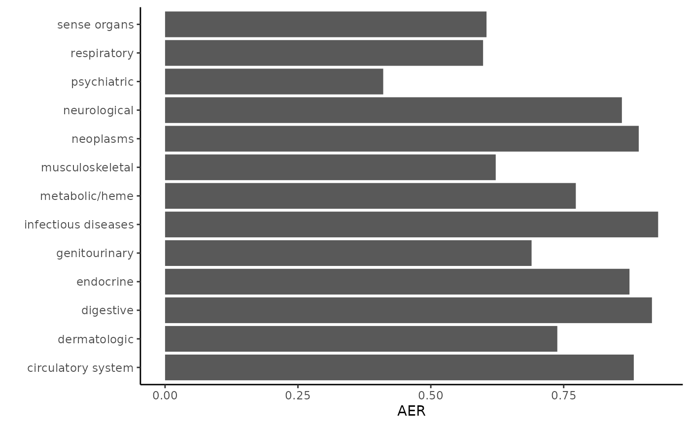
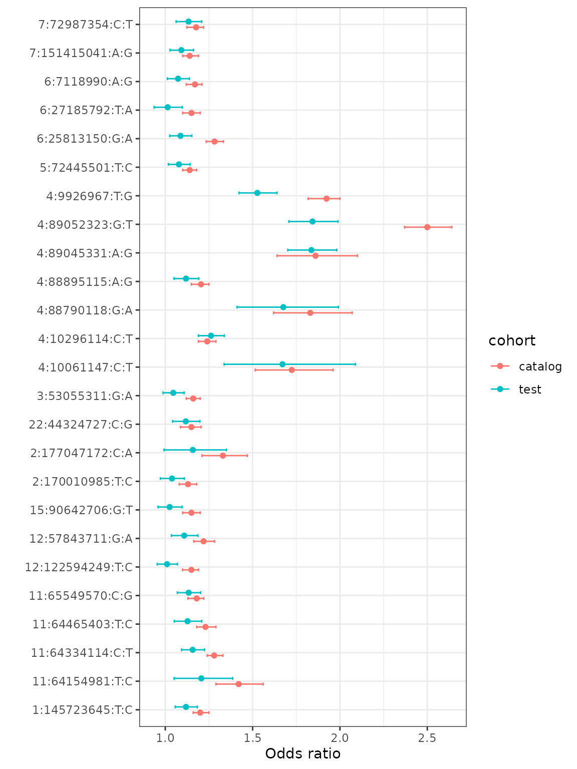
Comparing a single phenotype
You can also compare the associations for a single phenotype against what was reported in the catalog. To do this, we use the rOR, rL95, and rU95 values from the annotion file as columns have been oriented to the risk allele. To make a plot, we will bind results from the test cohort and the source cohort (catalog) for a single phenotype.
gout_test = anno[phecode_string %like% 'Gout',c('SNP', 'rOR', 'rL95', 'rU95')]
gout_test$cohort = 'test'
gout_cat = anno[phecode_string %like% 'Gout', c('SNP', 'cat_OR', 'cat_L95', 'cat_U95')]
gout_cat$cohort = 'catalog'
gout = rbind(gout_test, gout_cat, use.names = FALSE)

ggplot(gout, aes(y = SNP, x = rOR, color = cohort)) +
  geom_point(position = position_dodge(width = 0.4)) +
  geom_errorbar(aes(xmin = rL95, xmax = rU95), width = 0.2, position = position_dodge(width = 0.4)) +
  ylab('') + xlab('Odds ratio') + theme_bw()